1 Introduction
I already wrote about “Logistic Regression” and “Support Vector Machines”. I also showed how to optimize these linear classifiers using “SGD training” and how to use the “OneVersusRest and OneVersusAll” Classifier to convert binary classifiers to multiple classifiers. Let’s come to a further binary classifier: the Perceptron.
For this post the dataset Iris from the statistic platform “Kaggle” was used. You can download the dataset from my “GitHub Repository”.
2 Background information on Perceptron Algorithm
In machine learning, the perceptron is an algorithm for supervised learning of binary classifiers. It’s a type of linear classifier, i.e. a classification algorithm that makes its predictions based on a linear predictor function combining a set of weights with the feature vector.

Components:
Input: All the feature becomes the input for a perceptron. We denote the input of a perceptron by [x1, x2, x3, ..,xn], here x represent the feature value and n represent the total number of features.
Weights: Weights are the values that are computed over the time of training the model. Initial we start the value of weights with some initial value and these values get updated for each training error. We represent the weights for perceptron by [w1,w2,w3, ..,wn].
BIAS: A bias neuron allows a classifier to shift the decision boundary left or right. In an algebraic term, the bias neuron allows a classifier to translate its decision boundary and helps to training the model faster and with better quality.
Weighted Summation: Weighted Summation is the sum of value that we get after the multiplication of each weight [wn] associated the each feature value[xn].
Step/Activation Function: the role of activation functions is make neural networks non-linear. For linerarly classification of example, it becomes necessary to make the perceptron as linear as possible.
Output: The weighted Summation is passed to the step/activation function and whatever value we get after computation is our predicted output.
Procedure:
- Fistly the features for an examples given as input to the Perceptron.
- These input features get multiplied by corresponding weights [starts with initial value].
- Summation is computed for value we get after multiplication of each feature with corresponding weight.
- Value of summation is added to bias.
- Step/Activation function is applied to the new value.
3 Loading the libraries and the data
import numpy as np
import pandas as pd

import seaborn as sns

#For chapter 4
from sklearn.model_selection import train_test_split
from sklearn.metrics import accuracy_score
from sklearn.linear_model import Perceptron

#For chapter 5
from sklearn.model_selection import GridSearchCV

#For chapter 6
from sklearn.multiclass import OneVsRestClassifier
from sklearn.multiclass import OneVsOneClassifier

#For chapter 7
from sklearn.linear_model import SGDClassifier
4 Perceptron - Model Fitting and Evaluation
For the use of the perceptron, we first take only two variables from the iris data set (‘sepal_length’ and ‘sepal_width’) and only two iris types (‘Iris-setosa’ and ‘Iris-virginica’).
iris = pd.read_csv("Iris_Data.csv")
iris = iris[['sepal_length', 'sepal_width', 'species']]
iris = iris[(iris["species"] != 'Iris-versicolor')]
print(iris['species'].value_counts().head().T)
print()
print('------------------------------------------')
print()
print(iris.head())
Let’s plot them:
ax = sns.scatterplot(x="sepal_length", y="sepal_width", hue="species", data=iris)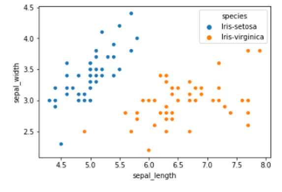
Now let’s split the data and train the model as well as evaluate it.
x = iris.drop('species', axis=1)
y = iris['species']
trainX, testX, trainY, testY = train_test_split(x, y, test_size = 0.2)
clf = Perceptron()
clf.fit(trainX, trainY)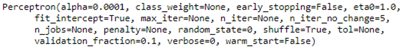
y_pred = clf.predict(testX)

print('Accuracy: {:.2f}'.format(accuracy_score(testY, y_pred)))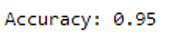
Wow 95% accuracy with the perceptron as binary classifier.
5 Hyperparameter optimization via Grid Search
Now we are trying to improve the model performance using grid search.
param_grid = {"alpha": [0.0001, 0.0003, 0.001, 0.003, 0.01, 0.03, 0.1, 0.3],
              "n_iter": [5, 10, 15, 20, 50],
              }

grid = GridSearchCV(clf, param_grid, cv=10, scoring='accuracy')

grid.fit(trainX, trainY)
print(grid.best_score_)
print(grid.best_params_)
6 OvO/OvR with the Perceptron
To show OvR and OvO using Perceptron, the iris data set is loaded again. This time without restrictions or filters.
iris = pd.read_csv("Iris_Data.csv")x = iris.drop('species', axis=1)
y = iris['species']
trainX, testX, trainY, testY = train_test_split(x, y, test_size = 0.2)OvR
OvR_clf = OneVsRestClassifier(Perceptron())
OvR_clf.fit(trainX, trainY)

y_pred = OvR_clf.predict(testX)

print('Accuracy of OvR Classifier: {:.2f}'.format(accuracy_score(testY, y_pred)))
OvO
OvO_clf = OneVsOneClassifier(Perceptron())
OvO_clf.fit(trainX, trainY)

y_pred = OvO_clf.predict(testX)

print('Accuracy of OvO Classifier: {:.2f}'.format(accuracy_score(testY, y_pred)))
As we can see, OvR doesn’t work quite as well but OvO does.
7 Perceptron with SGD training
Finally I show how to use the Perceptron with SGD training. For this we reload the iris data set as already done in chapter 4.
iris = pd.read_csv("Iris_Data.csv")
iris = iris[['sepal_length', 'sepal_width', 'species']]
iris = iris[(iris["species"] != 'Iris-versicolor')]
x = iris.drop('species', axis=1)
y = iris['species']
trainX, testX, trainY, testY = train_test_split(x, y, test_size = 0.2)clf = SGDClassifier(loss="perceptron", penalty="l2")
clf.fit(trainX, trainY)
y_pred = clf.predict(testX)
print('Accuracy: {:.2f}'.format(accuracy_score(testY, y_pred)))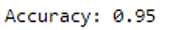
8 Conclusion
This post described how the Perceptron algorithm works and how it can be used in python. Furthermore, the model improvement via grid search was discussed as well as the use of OvR and OvO to convert the binary classifier into a multiple.