1 Introduction
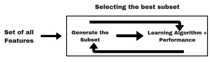
Image Source: “Analytics Vidhya”
Embedded methods are iterative in a sense that takes care of each iteration of the model training process and carefully extract those features which contribute the most to the training for a particular iteration. Regularization methods are the most commonly used embedded methods which penalize a feature given a coefficient threshold.
Regularization is a technique which makes slight modifications to the learning algorithm such that the model generalizes better. L1 (LASSO) and L2 (Ridge) are the most common types of regularization. These update the general cost function by adding another term known as the regularization term. In addition to ridge and lasso, another embedded method will be shown in this post: Elastic Net. This is a combination between a lasso and a ridge regression.
For this post the dataset Auto-mpg from the statistic platform “Kaggle” was used. You can download it from my GitHub Repository.
2 Loading the libraries and the data
import numpy as np
import pandas as pd


from sklearn.model_selection import train_test_split
from sklearn import metrics
from sklearn.preprocessing import StandardScaler

from sklearn.linear_model import LinearRegression
from sklearn.linear_model import Ridge
from sklearn.linear_model import Lasso
from sklearn.linear_model import ElasticNet

import matplotlib.pyplot as plt

from sklearn.model_selection import GridSearchCV
from sklearn.pipeline import Pipeline
cars = pd.read_csv("auto-mpg.csv")
cars["horsepower"] = pd.to_numeric(cars.horsepower, errors='coerce')
cars_horsepower_mean = cars['horsepower'].fillna(cars['horsepower'].mean())
cars['horsepower'] = cars_horsepower_mean
cars.head()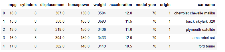
For a better performance of the algorithms it is always advisable to scale the predictors. The ridge, lasso and elastic net algithithm from scikit learn have a built-in function for this. Have a look “here” for further information.
#Selection of the predictors and the target variable
x = cars.drop(['mpg', 'car name'], axis = 1)
y = cars["mpg"]

#Scaling of the features
col_names = x.columns
features = x[col_names]

scaler = StandardScaler().fit(features.values)
features = scaler.transform(features.values)
scaled_features_x = pd.DataFrame(features, columns = col_names)
scaled_features_x.head()

#Train Test Split
trainX, testX, trainY, testY = train_test_split(scaled_features_x, y, test_size = 0.2)
3 Embedded methods
In short, ridge regression and lasso are regression techniques optimized for prediction, rather than inference. Normal regression gives you unbiased regression coefficients. Ridge and lasso regression allow you to regularize (shrink) coefficients. This means that the estimated coefficients are pushed towards 0, to make them work better on new data-sets. This allows you to use complex models and avoid over-fitting at the same time.
For both ridge and lasso you have to set a so called meta-parameter that defines how aggressive regularization is performed. Meta-parameters are usually chosen by cross-validation. For Ridge regression the meta-parameter is often called alpha or L2; it simply defines regularization strength. For LASSO the meta-parameter is often called lambda, or L1. In contrast to Ridge, the LASSO regularization will actually set less-important predictors to 0 and help you with choosing the predictors that can be left out of the model. The two methods are combined in Elastic Net Regularization. Here, both parameters can be set, with L2 defining regularization strength and L1 the desired sparseness of results.
First of all let’s start with a simple linear regression model. If you are not familiar yet with linear regression and its parameter and metrics have a look “here”
lm = LinearRegression()
lm.fit(trainX, trainY)

print('Training score (R²): {}'.format(lm.score(trainX, trainY)))
print('Test score (R²): {}'.format(lm.score(testX, testY)))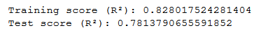
y_pred = lm.predict(testX)

print('Mean Absolute Error:', metrics.mean_absolute_error(testY, y_pred))
print('Mean Squared Error:', metrics.mean_squared_error(testY, y_pred))
print('Root Mean Squared Error:', np.sqrt(metrics.mean_squared_error(testY, y_pred)))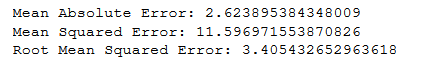
lm_coef = lm.coef_
df = list(zip(col_names, lm_coef))
df = pd.DataFrame(df, columns=['Features', 'Coefficient'])
df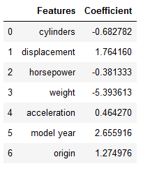
For a quick overview of the strengths of the individual coefficients it is good to visualize them.
plt.figure(figsize = (8,6))
coef_plot = pd.Series(lm.coef_, index = col_names)
coef_plot.plot(kind='barh')
plt.title('Simple linear regression')
plt.xlabel('Coefficients')
plt.ylabel('Predictors')
plt.show()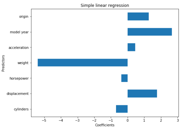
3.1 Ridge Regression
The ridge regression syntax (as well as those of lasso and elastic net) is analogous to linear regression. Here are two short sentences about how ridge works:
- It shrinks the parameters, therefore it is mostly used to prevent multicollinearity.
- It reduces the model complexity by coefficient shrinkage.
ridge_reg = Ridge(alpha=10, fit_intercept=True)

ridge_reg.fit(trainX, trainY)

print('Training score (R²): {}'.format(ridge_reg.score(trainX, trainY)))
print('Test score (R²): {}'.format(ridge_reg.score(testX, testY)))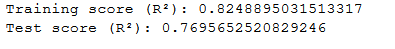
y_pred = ridge_reg.predict(testX)

print('Mean Absolute Error:', metrics.mean_absolute_error(testY, y_pred))
print('Mean Squared Error:', metrics.mean_squared_error(testY, y_pred))
print('Root Mean Squared Error:', np.sqrt(metrics.mean_squared_error(testY, y_pred)))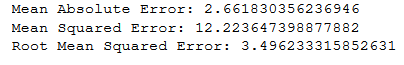
ridge_coef = ridge_reg.coef_
df = list(zip(col_names, ridge_coef))
df = pd.DataFrame(df, columns=['Features', 'Coefficient'])
df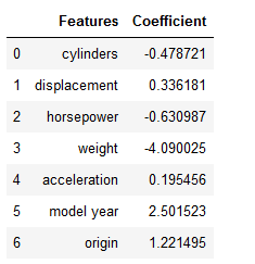
Next to the metrics of performance, we plot the strengths of the individual coefficients again. Here are two ways to do so.
# Plot the coefficients
plt.plot(range(len(col_names)), ridge_coef)
plt.xticks(range(len(col_names)), col_names.values, rotation=60)
plt.margins(0.02)
plt.show()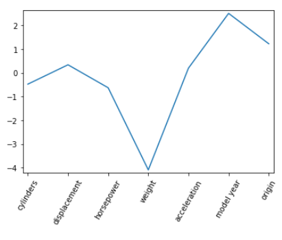
plt.figure(figsize = (8,6))
coef_plot = pd.Series(ridge_reg.coef_, index = col_names)
coef_plot.plot(kind='barh')
plt.title('Ridge regression')
plt.xlabel('Coefficients')
plt.ylabel('Predictors')
plt.show()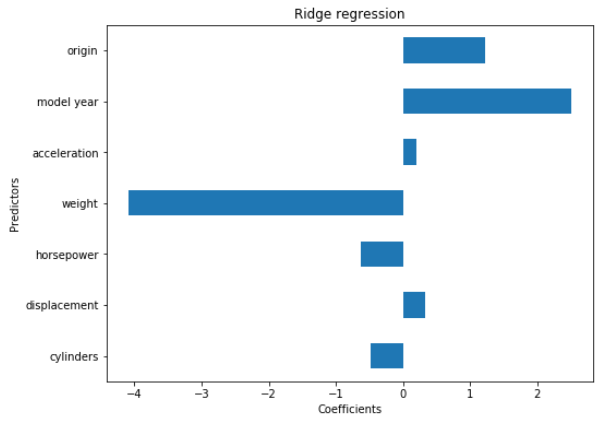
3.2 Lasso Regression
Lasso Regression is generally used when we have more number of features, because it automatically does feature selection.
lasso_reg = Lasso(alpha=0.3, fit_intercept=True)

lasso_reg.fit(trainX, trainY)

print('Training score (R²): {}'.format(lasso_reg.score(trainX, trainY)))
print('Test score (R²): {}'.format(lasso_reg.score(testX, testY)))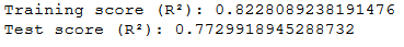
y_pred = lasso_reg.predict(testX)

print('Mean Absolute Error:', metrics.mean_absolute_error(testY, y_pred))
print('Mean Squared Error:', metrics.mean_squared_error(testY, y_pred))
print('Root Mean Squared Error:', np.sqrt(metrics.mean_squared_error(testY, y_pred)))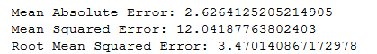
lasso_coef = lasso_reg.coef_
df = list(zip(col_names, lasso_coef))
df = pd.DataFrame(df, columns=['Features', 'Coefficient'])
df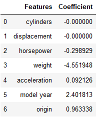
# Plot the coefficients
plt.plot(range(len(col_names)), lasso_coef)
plt.xticks(range(len(col_names)), col_names.values, rotation=60)
plt.margins(0.02)
plt.show()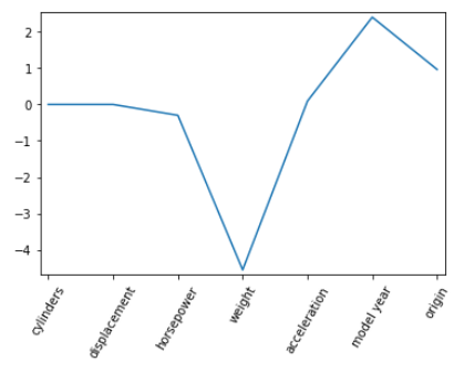
plt.figure(figsize = (8,6))
coef_plot = pd.Series(lasso_reg.coef_, index = col_names)
coef_plot.plot(kind='barh')
plt.title('Lasso regression')
plt.xlabel('Coefficients')
plt.ylabel('Predictors')
plt.show()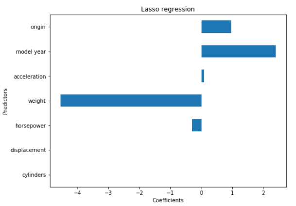
3.3 Elastic Net
Elastic Net is a combination of ridge regression and lasso regression.
ElaNet_reg = ElasticNet()

ElaNet_reg.fit(trainX, trainY)

print('Training score (R²): {}'.format(lasso_reg.score(trainX, trainY)))
print('Test score (R²): {}'.format(lasso_reg.score(testX, testY)))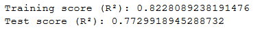
y_pred = ElaNet_reg.predict(testX)

print('Mean Absolute Error:', metrics.mean_absolute_error(testY, y_pred))
print('Mean Squared Error:', metrics.mean_squared_error(testY, y_pred))
print('Root Mean Squared Error:', np.sqrt(metrics.mean_squared_error(testY, y_pred)))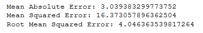
ElaNet_coef = ElaNet_reg.coef_
df = list(zip(col_names, ElaNet_coef))
df = pd.DataFrame(df, columns=['Features', 'Coefficient'])
df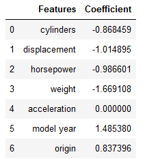
# Plot the coefficients
plt.plot(range(len(col_names)), ElaNet_coef)
plt.xticks(range(len(col_names)), col_names.values, rotation=60)
plt.margins(0.02)
plt.show()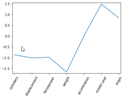
plt.figure(figsize = (8,6))
coef_plot = pd.Series(ElaNet_reg.coef_, index = col_names)
coef_plot.plot(kind='barh')
plt.title('Lasso regression')
plt.xlabel('Coefficients')
plt.ylabel('Predictors')
plt.show()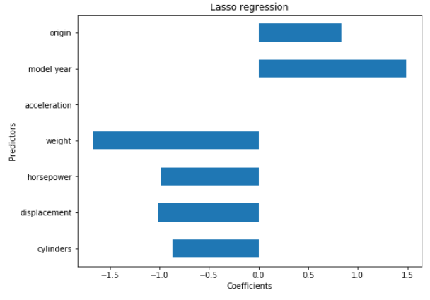
4 Grid Search
Grid search is an approach to parameter tuning that will methodically build and evaluate a model for each combination of algorithm parameters specified in a grid.
4.1 Grid for Ridge
The code below evaluates different alpha values for the Ridge Regression.
ridge_reg = Ridge()

param_grid = [{'alpha':[1e-15, 1e-10, 1e-8, 1e-4, 1e-3,1e-2, 1, 2, 5, 7, 10, 15, 20]}]

grid = GridSearchCV(ridge_reg, param_grid, cv = 10)

grid.fit(trainX, trainY)
print(grid.best_score_)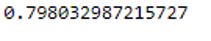
print(grid.best_params_) 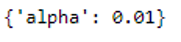
We see that the result from grid search is worse than that from the original model.Something like that can happen. It does not matter anyway.
4.2 Grid for embedded methods
We also can use Grid Search to compare all embedded methods with the different values for alpha:
ridge_reg = Ridge()
lasso_reg = Lasso()
ElaNet_reg = ElasticNet()


# Just initialize the pipeline with any estimator you like
pipe = Pipeline(steps=[('estimator', Ridge())])

# Add a dict of estimator and estimator related parameters in this list
params_grid = [{
                'estimator':[Ridge()],
                'estimator__alpha': [1e-15, 1e-10, 1e-8, 1e-4, 1e-3,1e-2, 1, 2, 5, 7, 10, 15, 20]
                },
                {
                'estimator':[Lasso()],
                'estimator__alpha': [1e-15, 1e-10, 1e-8, 1e-4, 1e-3,1e-2, 1, 2, 5, 7, 10, 15, 20]
                },
                {
                'estimator': [ElasticNet()],
                'estimator__alpha': [1e-15, 1e-10, 1e-8, 1e-4, 1e-3,1e-2, 1, 2, 5, 7, 10, 15, 20]
                }
              ]

grid = GridSearchCV(pipe, params_grid, cv=5)

grid.fit(trainX, trainY)

print(grid.best_params_) 
5 Conclusion
Within my latest post “Wrapper methods” I described how they work and how they are differentiated from filter methods. But what’s the difference between wrapper methods and embedded methods?
The difference from embedded methods to wrapper methods is that an intrinsic model building metric is used during learning. Furthermore embedded methods use algorithms that have built-in feature selection methods.
I also gave this overview of the three types of feature selection:
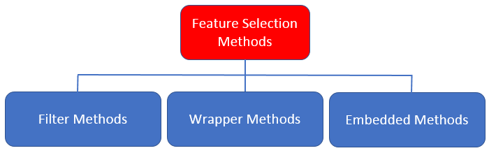
Let’s summarize again…
In previous publications we treated filter methods:
Then we went over to the wrapper methods:
Finally we showed in this post the three best known embedded methods work.
In addition to the explained syntax, the delimitation of the methods was also discussed.
Typical Use Cases
- Ridge: It is majorly used to prevent overfitting. Since it includes all the features, it is not very useful in case of exorbitantly high #features, say in millions, as it will pose computational challenges.
- Lasso: Since it provides sparse solutions, it is generally the model of choice (or some variant of this concept) for modelling cases where the #features are in millions or more. In such a case, getting a sparse solution is of great computational advantage as the features with zero coefficients can simply be ignored.