1 Introduction
Next to “higly correlated” and “constant” features outlier detection is also a central element of data pre-processing.
In statistics, outliers are data points that do not belong to any particular population.
In the following three methods of outlier detection are presented.
2 Loading the libraries
import numpy as np
import pandas as pd
import seaborn as sns
import matplotlib.pyplot as plt
3 Boxplots - Method
df = pd.DataFrame({'name': ['Anton', 'Susi', 'Moni', 'Renate', 'Otto', 'Karl', 'Sven', 'Sandra', 'Svenja', 'Karl', 'Karsten'],
                   'age': [24,22,30,21,20,23,22,20,24,20,22],
                   'salary': [4700,2400,4500,2500,3000,2700,3200,4000,7500,3600,2800]})
df
A very simple way to recognize outlier is to use boxplots. We pay attention to data points that are outside the upper and lower whiskers.
sns.boxplot(data=df['age'])
sns.boxplot(data=df['salary'])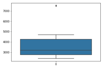
4 Z-score method
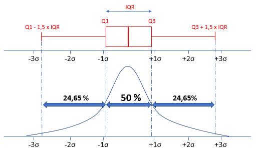
In statistics, if a data distribution is approximately normal then about 68% of the data points lie within one standard deviation (sd) of the mean and about 95% are within two standard deviations, and about 99.7% lie within three standard deviations.
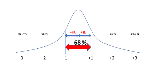
Therefore, if you have any data point that is more than 3 times the standard deviation, then those points are very likely to be outliers.
df = pd.DataFrame({'name': ['Anton', 'Susi', 'Moni', 'Renate', 'Otto', 'Karl', 'Sven', 'Sandra', 'Svenja', 'Karl', 'Karsten'],
                   'age': [24,22,138,21,20,23,22,30,24,20,22],
                   'salary': [4700,2400,4500,2500,3000,2700,3200,4000,150000,3600,2800]})
df
df.shape
Let’s define the function:
def outliers_z_score(df):
    threshold = 3

    mean = np.mean(df)
    std = np.std(df)
    z_scores = [(y - mean) / std for y in df]
    return np.where(np.abs(z_scores) > threshold)
For the further proceeding we just need numerical colunns:
my_list = ['int16', 'int32', 'int64', 'float16', 'float32', 'float64']
num_columns = list(df.select_dtypes(include=my_list).columns)
numerical_columns = df[num_columns]
numerical_columns.head(3)
Now we apply the defined function to all numerical columns:
outlier_list = numerical_columns.apply(lambda x: outliers_z_score(x))
outlier_list
To get our dataframe tidy, we have to create a list with the detected outliers and remove them from the original dataframe.
df_of_outlier = outlier_list.iloc[0]
df_of_outlier = pd.DataFrame(df_of_outlier)
df_of_outlier.columns = ['Rows_to_exclude']
df_of_outlier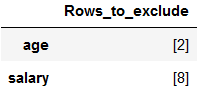
outlier_list_final = df_of_outlier['Rows_to_exclude'].to_numpy()
outlier_list_final
outlier_list_final = np.concatenate( outlier_list_final, axis=0 )
outlier_list_final
filter_rows_to_excluse = df.index.isin(outlier_list_final)

df_without_outliers = df[~filter_rows_to_excluse]

df_without_outliers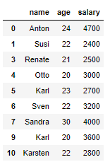
df_without_outliers.shape
As we can see the two outliers were removed from the dataframe.
print('Length of original dataframe: ' + str(len(df)))

print('Length of new dataframe without outliers: ' + str(len(df_without_outliers)))
print('----------------------------------------------------------------------------------------------------')
print('Difference between new and old dataframe: ' + str(len(df) - len(df_without_outliers)))
print('----------------------------------------------------------------------------------------------------')
print('Length of unique outlier list: ' + str(len(outlier_list_final)))
Important!
I recommend, if you remove outlier before a train test split when developing machine learning algorithms, that the index of the newly generated records is reassigned, otherwise you might have problems with joining.
5 IQR method
In addition to the Z-score method, outliers can also be identified using the IQR method. Here we look at which data points are outside the whiskers. This method has the advantage, that it uses robust parameters for the calculation.
df = pd.DataFrame({'name': ['Anton', 'Susi', 'Moni', 'Renate', 'Otto', 'Karl', 'Sven', 'Sandra', 'Svenja', 'Karl', 'Karsten'],
                   'age': [24,22,138,21,20,23,22,30,24,20,22],
                   'salary': [4700,2400,4500,2500,3000,2700,3200,4000,150000,3600,2800]})
df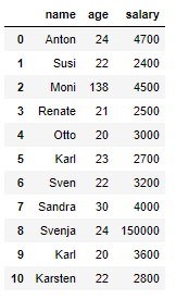
df.shape
5.1 Detect outlier for column ‘age’
column_to_be_examined = df['age']sorted_list = sorted(column_to_be_examined)q1, q3= np.percentile(sorted_list,[25,75])
print(q1)
print(q3)
iqr = q3 - q1
print(iqr)
lower_bound = q1 -(1.5 * iqr)
upper_bound = q3 +(1.5 * iqr)

print(lower_bound)
print(upper_bound)
outlier_col_age = df[(column_to_be_examined < lower_bound) | (column_to_be_examined > upper_bound)]
outlier_col_age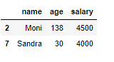
5.2 Detect outlier for column ‘salary’
column_to_be_examined = df['salary']
sorted_list = sorted(column_to_be_examined)
q1, q3= np.percentile(sorted_list,[25,75])
iqr = q3 - q1
lower_bound = q1 -(1.5 * iqr)
upper_bound = q3 +(1.5 * iqr)
outlier_col_salary = df[(column_to_be_examined < lower_bound) | (column_to_be_examined > upper_bound)]
outlier_col_salary
5.3 Remove outlier from dataframe
outlier_col_age = outlier_col_age.reset_index()
outlier_list_final_col_age = outlier_col_age['index'].tolist()
outlier_list_final_col_age
outlier_col_salary = outlier_col_salary.reset_index()
outlier_list_final_col_salary = outlier_col_salary['index'].tolist()
outlier_list_final_col_salary
outlier_list_final = np.concatenate((outlier_list_final_col_age, outlier_list_final_col_salary), axis=None)
outlier_list_final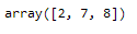
filter_rows_to_exclude = df.index.isin(outlier_list_final)

df_without_outliers = df[~filter_rows_to_exclude]

df_without_outliers
df_without_outliers.shape
6 Conclusion
Outlier in a dataframe can lead to strong distortions in predictions. It is therefore essential to examine your data for outlier or influential values before training machine learning models.