1 Introduction
2 Loading the libraries and the data
3 Preparation
4 Correlations with the output variable
5 Identification of highly correlated features
6 Removing highly correlated features
- 6.1 Selecting numerical variables
- 6.2 Train / Test Split
7 Conclusion

1 Introduction

One of the points to remember about data pre-processing for regression analysis is multicollinearity. This post is about finding highly correlated predictors within a dataframe.

For this post the dataset Auto-mpg from the statistic platform “Kaggle” was used. You can download it from my GitHub Repository.

2 Loading the libraries and the data

import pandas as pd
import numpy as np
import matplotlib
import matplotlib.pyplot as plt
import seaborn as sns
from sklearn.model_selection import train_test_split
from sklearn.feature_selection import VarianceThreshold

cars = pd.read_csv("path/to/file/auto-mpg.csv")

3 Preparation

# convert categorial variables to numerical
# replace missing values with columns'mean

cars["horsepower"] = pd.to_numeric(cars.horsepower, errors='coerce')
cars_horsepower_mean = cars['horsepower'].fillna(cars['horsepower'].mean())
cars['horsepower'] = cars_horsepower_mean

When we talk about correlation it’s easy to get a first glimpse with a heatmap:

plt.figure(figsize=(8,6))
cor = cars.corr()
sns.heatmap(cor, annot=True, cmap=plt.cm.Reds)
plt.show()

Definition of the predictors and the criterion:

predictors = cars.drop(['mpg', 'car name'], axis = 1) 
criterion = cars["mpg"]

predictors.head()

4 Correlations with the output variable

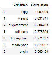
To get an idea which Variables maybe import for our model:

threshold = 0.5


cor_criterion = abs(cor["mpg"])

relevant_features = cor_criterion[cor_criterion>threshold]
relevant_features = relevant_features.reset_index()
relevant_features.columns = ['Variables', 'Correlation']
relevant_features = relevant_features.sort_values(by='Correlation', ascending=False)
relevant_features

5 Identification of highly correlated features

One model assumption of linear regression analysis is to avoid multicollinearity. This function is to find high correlations:

threshold = 0.8

def high_cor_function(df):
    cor = df.corr()
    corrm = np.corrcoef(df.transpose())
    corr = corrm - np.diagflat(corrm.diagonal())
    print("max corr:",corr.max(), ", min corr: ", corr.min())
    c1 = cor.stack().sort_values(ascending=False).drop_duplicates()
    high_cor = c1[c1.values!=1]    
    thresh = threshold 
    display(high_cor[high_cor>thresh])

high_cor_function(predictors)

6 Removing highly correlated features

6.1 Selecting numerical variables

cars.shape

Here we see that the dataframe ‘cars’ originaly have 9 columns and 398 observations. With the following snippet we just select numerical variables:

num_col = ['int16', 'int32', 'int64', 'float16', 'float32', 'float64']
numerical_columns = list(cars.select_dtypes(include=num_col).columns)
cars_data = cars[numerical_columns]

cars_data.head()

cars_data.shape

As you can see, one column (Here ‘car name’) were dropped.

6.2 Train / Test Split

It is important to mention here that, in order to avoid overfitting, feature selection should only be applied to the training set.

x = cars_data.drop('mpg', axis=1)
y = cars_data['mpg']
trainX, testX, trainY, testY = train_test_split(x, y, test_size = 0.2)

correlated_features = set()
correlation_matrix = cars_data.corr()

threshold = 0.90

for i in range(len(correlation_matrix .columns)):
    for j in range(i):
        if abs(correlation_matrix.iloc[i, j]) > threshold:
            colname = correlation_matrix.columns[i]
            correlated_features.add(colname)

Number of columns in the dataset, with correlation value of greater than 0.9 with at least 1 other column:

len(correlated_features)

With the following code we receive the names of these features:

print(correlated_features)

Finally, the identified features are excluded:

trainX_clean = trainX.drop(labels=correlated_features, axis=1)
testX_clean = testX.drop(labels=correlated_features, axis=1)



# Even possibe without assignment to a specific object:

## trainX.drop(labels=correlated_features, axis=1, inplace=True)
## testX.drop(labels=correlated_features, axis=1, inplace=True)

7 Conclusion

This post has shown, how to identify highly correlated variables and exclude them for further use.

Dealing with highly correlated features