- 1 Introduction
- 2 Loading the Libraries and the Data
- 3 Checking for missing values
- 4 Droping of Missing Values
- 5 Imputations
- 6 Further Imputation Methods
- 7 KNNImputer
- 8 Imputation in Practice
- 9 Conclusion
1 Introduction
In the real world, there is virtually no record that has no missing values. Dealing with missing values can be done differently. In the following several methods will be presented how to deal with them.
2 Loading the Libraries and the Data
import pandas as pd
import numpy as np

from sklearn.impute import SimpleImputer
from sklearn.pipeline import Pipeline

from sklearn.impute import KNNImputer

from sklearn.model_selection import train_test_split
import pickle as pk
import random
df = pd.DataFrame({'Name': ['Anton', 'Moni', np.NaN, 'Renate', 'Justus'],
'Age': [32,22,62,np.NaN,18],
'Salary': [np.NaN, np.NaN,4500,2500,3800],
'Job': ['Student', np.NaN, 'Manager', 'Teacher', 'Student']})
df
3 Checking for missing values
df.isnull().sum()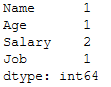
def mv_overview_func(df):
    '''
    Gives an overview of the total number and percentage of missing values in a data set

    Args:
        df (DataFrame): Dataframe to which the function is to be applied

    Returns:
        Overview of the total number and percentage of missing values
    '''
    # Total missing values
    mis_val = df.isnull().sum()
    # Percentage of missing values
    mis_val_percent = 100 * df.isnull().sum() / len(df)
    # Data Types
    data_types = df.dtypes
    # Make a table with the results
    mis_val_table = pd.concat([mis_val, mis_val_percent, data_types], axis=1)
    # Rename the columns
    mis_val_table_ren_columns = mis_val_table.rename(
    columns = {0 : 'Missing Values', 1 : '% of Total Values', 2 : 'Data Type'})
    # Sort the table by percentage of missing descending
    mis_val_table_ren_columns = mis_val_table_ren_columns[
        mis_val_table_ren_columns.iloc[:,1] != 0].sort_values(
        '% of Total Values', ascending=False).round(1)
    # Print some summary information
    print ("Your selected dataframe has " + str(df.shape[1]) + " columns.\n"
            "There are " + str(mis_val_table_ren_columns.shape[0]) +
            " columns that have missing values.")
    # Return the dataframe with missing information
    return mis_val_table_ren_columns
mv_overview_func(df)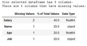
4 Droping of Missing Values
df_drop = df.copy()
df_drop
All rows with minimum one NaN will be dropped:
df_drop.dropna()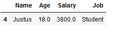
All rows from the defined columns with a NaN will be dropped:
df_drop.dropna(subset=['Name', 'Age'])
5 Imputations
5.1 for NUMERIC Features
5.1.1 Replace np.NaN with specific values
df_replace_1 = df.copy()
df_replace_1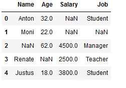
Missing values from only one column (here ‘Name’) are replaced:
df_replace_1['Name'] = df_replace_1['Name'].fillna(0)
df_replace_1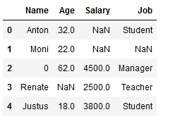
Missing values from the complete dataset will be replaced:
df_replace_1.fillna(0, inplace=True)
df_replace_1
Does that make sense? Probably not. So let’s look at imputations that follow a certain logic.
5.1.2 Replace np.NaN with MEAN
A popular metric for replacing missing values is the use of mean.
df_replace_2 = df.copy()
df_replace_2
df_replace_2['Age'].mean()
Here all missing values of the column ‘Age’ are replaced by their mean value.
df_replace_2['Age'] = df_replace_2['Age'].fillna(df_replace_2['Age'].mean())
df_replace_2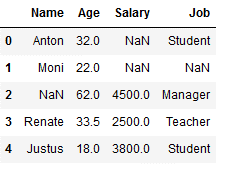
scikit-learn - SimpleImputer
Always keep in mind that you will need all the steps you take to prepare for model training to make predictions later.
What do I mean by that exactly? If the data set you have available for model training already has missing values, it is quite possible that future data sets for which predictions are to be made will also contain missing values. In order for the prediction model to work, these missing values must be replaced by metrics that were also used in the model training.
df_replace_3 = df.copy()
df_replace_3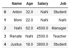
imp_age_mean = SimpleImputer(missing_values=np.nan, strategy='mean')

imp_age_mean.fit(df_replace_3[['Age']])
df_replace_3['Age'] = imp_age_mean.transform(df_replace_3[['Age']])
df_replace_3
In the steps shown before, I used the .fit and .transform functions separately. If it’s not about model training, you can also combine these two steps and save yourself another line of code.
df_replace_4 = df.copy()
df_replace_4
imp_age_mean = SimpleImputer(missing_values=np.nan, strategy='mean')

df_replace_4['Age'] = imp_age_mean.fit_transform(df_replace_4[['Age']])
df_replace_4
This way you can see which value is behind imp_age_mean concretely:
imp_age_mean.statistics_
5.1.3 Replace np.NaN with MEDIAN
Other metrics such as the median can also be used instead of missing values:
df_replace_5 = df.copy()
df_replace_5
imp_age_median = SimpleImputer(missing_values=np.nan, strategy='median')

df_replace_5['Age'] = imp_age_median.fit_transform(df_replace_5[['Age']])
df_replace_5
imp_age_median.statistics_
5.1.4 Replace np.NaN with most_frequent
For some variables, it makes sense to use the most frequently occurring value for NaNs instead of mean or median.
df_replace_6 = df.copy()
df_replace_6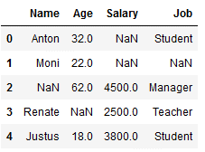
imp_age_mfreq = SimpleImputer(missing_values=np.nan, strategy='most_frequent')

df_replace_6['Age'] = imp_age_mfreq.fit_transform(df_replace_6[['Age']])
df_replace_6
Since there is no value in the variable ‘Age’ that occurs twice or more often, the lowest value is automatically taken. The same would apply if there were two equally frequent values.
5.2 for CATEGORICAL Features
5.2.1 Replace np.NaN with most_frequent
The most_frequent function can be used for numeric variables as well as categorical variables.
df_replace_7 = df.copy()
df_replace_7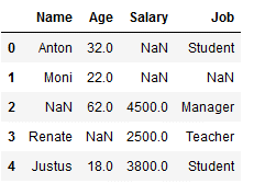
imp_job_mfreq = SimpleImputer(missing_values=np.nan, strategy='most_frequent')

df_replace_7['Job'] = imp_job_mfreq.fit_transform(df_replace_7[['Job']])
df_replace_7
Here we see that with a frequency of 2, the job ‘student’ is the most common, so this is used for the missing value here.
imp_job_mfreq.statistics_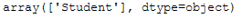
But what happens if we just don’t have a most frequent value in a categorical column like in our example within the column ‘Name’?
df_replace_8 = df.copy()
df_replace_8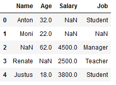
imp_name_mfreq = SimpleImputer(missing_values=np.nan, strategy='most_frequent')

df_replace_8['Name'] = imp_name_mfreq.fit_transform(df_replace_8[['Name']])
df_replace_8
Again, the principle that the lowest value is used applies. In our example, this is the name Anton, since it begins with A and thus comes before all other names in the alphabet.
5.2.2 Replace np.NaN with specific values
df_replace_9 = df.copy()
df_replace_9
However, we also have the option of using certain values:
imp_job_const = SimpleImputer(missing_values=np.nan,
                              strategy='constant',
                              fill_value='others')

df_replace_9['Job'] = imp_job_const.fit_transform(df_replace_9[['Job']])
df_replace_9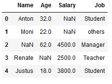
5.3 for specific Values
Not only a certain kind of values like NaN values can be replaced, this is also possible with specific values.
5.3.1 single values
For the following example we take the last version of the last used data set, here df_replace_9:
df_replace_9
rep_job_const = SimpleImputer(missing_values='others',
                              strategy='constant',
                              fill_value='not_in_scope')

df_replace_9['Job'] = rep_job_const.fit_transform(df_replace_9[['Job']])
df_replace_9
As we can see, ‘others’ became ‘not_in_scope’.
5.3.2 multiple values
Unfortunately, we cannot work with lists for multiple values. But with the use of the pipeline function it works. We use for our following example again the last state of the dataset ‘df_replace_9’:
rep_pipe = Pipeline([('si1',SimpleImputer(missing_values = 'Manager',
                                          strategy='constant',
                                          fill_value='not_relevant')),
                     ('si2', SimpleImputer(missing_values = 'Teacher',
                                           strategy='constant',
                                           fill_value='not_relevant'))])

df_replace_9['Job'] = rep_pipe.fit_transform(df_replace_9[['Job']])
df_replace_9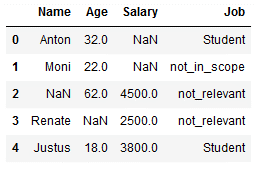
In my opinion, however, this approach has two disadvantages. Firstly, the values used are not saved (so cannot be reused automatically) and secondly, this is a lot of code to write. With an if-else function you would be faster:
def rep_func(col):

    if col == 'Student':
        return 'useless'
    if col == 'not_relevant':
        return 'useless'
    else:
        return 'useless'

df_replace_9['Job'] = df_replace_9['Job'].apply(rep_func)
df_replace_9
But again, the values used cannot be easily reused. You would have to create your own dictionary.
6 Further Imputation Methods
In the following chapter I would like to present some more imputation methods. They differ from the previous ones because they use different values instead of NaN values and not specific values as before.
In some cases, this can lead to getting a little closer to the truth and thus improve the model training.
6.1 with ffill
Here, the missing value is replaced by the preceding non-missing value.
df_replace_10 = df.copy()
df_replace_10
df_replace_10['Age'] = df_replace_10['Age'].fillna(method='ffill')
df_replace_10
The ffill function also works for categorical variables.
df_replace_10['Job'] = df_replace_10['Job'].fillna(method='ffill')
df_replace_10
The condition here is that there is a first value. Let’s have a look at the column ‘Salary’. Here we have two missing values right at the beginning. Here ffill does not work:
df_replace_10['Salary'] = df_replace_10['Salary'].fillna(method='ffill')
df_replace_10
6.2 with backfill
What does not work with ffill works with backfill. Backfill replaces the missing value with the upcoming non-missing value.
df_replace_10['Salary'] = df_replace_10['Salary'].fillna(method='backfill')
df_replace_10
6.3 Note on this Chapter
Due to the fact that different values are used for the missing values, it is not possible to define a uniform metric that should replace future missing values from the column.
However, one can proceed as follows for a model training. You start by using the functions ffill or backfill and then calculate a desired metric of your choice (e.g. mean) and save it for future missing values from the respective column.
I will explain the just described procedure in chapter 8.2 in more detail.
7 KNNImputer
Here, the KNN algorithm is used to replace missing values. If you want to know how KNN works exactly, check out this post of mine: Introduction to KNN Classifier. For this chapter, I have again created a sample data set:
df_knn = pd.DataFrame({'Name': ['Anton', 'Moni', 'Sven', 'Renate', 'Justus',
                                'Sarah', 'Jon', 'Alex', 'Jenny', 'Jo'],
                       'Age': [32,22,62,np.NaN,18,63,np.NaN,44,23,71],
                       'Salary': [4000, np.NaN,4500,2500,3800,5500,7000,np.NaN,4800,3700]})
df_knn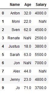
7.1 on single columns
df_knn_1 = df_knn.copy()


imp_age_knn = KNNImputer(n_neighbors=2)

df_knn_1['Age'] = imp_age_knn.fit_transform(df_knn_1[['Age']])
df_knn_1
imp_salary_knn = KNNImputer(n_neighbors=2)

df_knn_1['Salary'] = imp_salary_knn.fit_transform(df_knn_1[['Salary']])
df_knn_1
So far so good. However, this is not how the KNNImputer is used in practice. I will show you why in the following chapter.
7.2 on multiple columns
df_knn_2 = df_knn.copy()
df_knn_2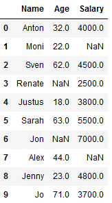
imp_age_salary_knn = KNNImputer(n_neighbors=2)

df_knn_2[['Age', 'Salary']] = imp_age_salary_knn.fit_transform(df_knn_2[['Age', 'Salary']])
df_knn_2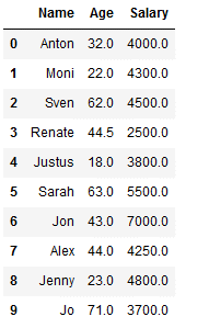
As you can see from the comparison below, the two methods use different values from the KNNImputer (see index 1,3 and 7).
print()
print('df_knn_1')
print()
print(df_knn_1)
print('-------------------------')
print()
print('df_knn_2')
print()
print(df_knn_2)
It should be mentioned here that sometimes it is better to choose this statistical approach in order to achieve better results in the later model training.
7.3 Note on this Chapter
KNNImputer stores the calculated metrics for each column added to it. The number and the order of the columns must remain the same!
8 Imputation in Practice
As already announced, I would like to show again how I use the replacement of missing values in practice during model training. It should be noted that I use a simple illustrative example below. In practice, there would most likely be additional steps like using encoders or feature scaling. This will be omitted at this point. But I will show in which case which order should be followed.
In the following, I use a modified version of the created dataset from the KNN example:
df_practice = df_knn.copy()
Target_Var = [0,0,1,0,1,1,0,1,1,0]
df_practice['Target_Var'] = Target_Var

df_practice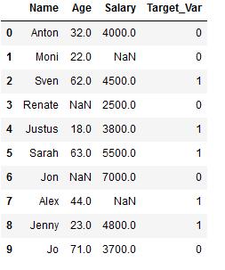
8.1 SimpleImputer in Practice
8.1.1 Train-Test Split
df_practice_simpl_imp = df_practice.copy()
df_practice_simpl_imp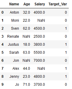
In model training, I first divide the data set into a training part and a test part.
x = df_practice_simpl_imp.drop('Target_Var', axis=1)
y = df_practice_simpl_imp['Target_Var']

trainX, testX, trainY, testY = train_test_split(x, y, test_size = 0.2)
print()
print('trainX')
print()
print(trainX)
print('-------------------------')
print()
print('testX')
print()
print(testX)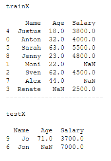
8.1.2 Fit&Transform (trainX)
Then I check if there are any Missing Values in trainX.
trainX.isnull().sum()
As we can see, we need to replace missing values in the columns ‘Age’ and ‘Salary’. For this I use the SimpleImputer with the strategy=‘mean’.
# Fit and Transform trainX column 'Age' with strategy='mean'
imp_age_mean1 = SimpleImputer(missing_values=np.nan, strategy='mean')
imp_age_mean1.fit(trainX[['Age']])
trainX['Age'] = imp_age_mean1.transform(trainX[['Age']])

# Fit and Transform trainX column 'Salary' with strategy='mean'
imp_salary_mean1 = SimpleImputer(missing_values=np.nan, strategy='mean')
imp_salary_mean1.fit(trainX[['Salary']])
trainX['Salary'] = imp_salary_mean1.transform(trainX[['Salary']])

print(trainX)
print()
print('Number of missing values:')
print(trainX.isnull().sum())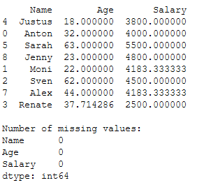
When I use the SimpleImputer, I save it separately to be able to use it again later.
pk.dump(imp_age_mean1, open('imp_age_mean1.pkl', 'wb'))
pk.dump(imp_salary_mean1, open('imp_salary_mean1.pkl', 'wb'))
8.1.3 Model Training
I won’t do the model training at this point, because that would still require me to either remove the categorical variable ‘name’ or convert it to a numeric one. This would only cause confusion at this point. Let’s assume we have done the model training like this.
dt = DecisionTreeClassifier()
dt.fit(trainX, trainY)
The execution of the prediction function (apart from the still existing categorical variable) would not work like this.
y_pred = df.predict(testX)Because we also have Missing Values in the testX part.
testX.isnull().sum()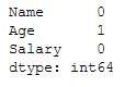
In order to be able to test the created model, we also need to replace them. For this purpose, we saved the metrics of the two SimpleImputers used in the previous step and can use them again here.
8.1.4 Transform (testX)
In the following, I will show the syntax to replace missing values for both columns (‘Age’ and ‘Salary’). I am aware that in this example only the ‘Age’ column contains a missing value. But in practice the data sets are usually larger than 10 observations.
# Transform testX column 'Age'
testX['Age'] = imp_age_mean1.transform(testX[['Age']])

# Transform testX column 'Salary'
testX['Salary'] = imp_salary_mean1.transform(testX[['Salary']])

print(testX)
print()
print('Number of missing values:')
print(testX.isnull().sum())
Now the test of our model training would also work.
8.2 ffill & backfill in Practice
As already noted in chapter 6.3, we cannot directly save a metric for further use with the ffill or backfill method. Therefore, in this part I show how I proceed in such a situation.
Here I will not go into each step individually, as they have been sufficiently explained in the previous chapter.
8.2.1 Train-Test Split
df_practice_ffill_bfill = df_practice.copy()
df_practice_ffill_bfill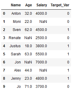
x = df_practice_ffill_bfill.drop('Target_Var', axis=1)
y = df_practice_ffill_bfill['Target_Var']

trainX, testX, trainY, testY = train_test_split(x, y, test_size = 0.2)
print()
print('trainX')
print()
print(trainX)
print('-------------------------')
print()
print('testX')
print()
print(testX)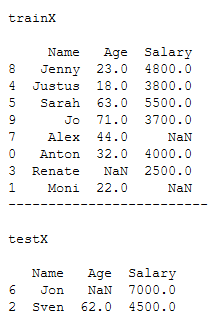
8.2.2 Use ffill or backfill
Now I will replace the missing values in our example with the ffill method.
# ffill column 'Age'
trainX['Age'] = trainX['Age'].fillna(method='ffill')
# ffill column 'Salary'
trainX['Salary'] = trainX['Salary'].fillna(method='ffill')

print(trainX)
print()
print('Number of missing values:')
print(trainX.isnull().sum())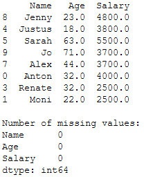
8.2.3 Fit (trainX)
# Fit trainX column 'Age' with strategy='mean'
imp_age_mean2 = SimpleImputer(missing_values=np.nan, strategy='mean')
imp_age_mean2.fit(trainX[['Age']])

# Fit trainX column 'Salary' with strategy='mean'
imp_salary_mean2 = SimpleImputer(missing_values=np.nan, strategy='mean')
imp_salary_mean2.fit(trainX[['Salary']])
pk.dump(imp_age_mean, open('imp_age_mean2.pkl', 'wb'))
pk.dump(imp_salary_mean, open('imp_salary_mean2.pkl', 'wb'))8.2.4 Transform (testX)
I’ll leave out the part about model training at this point, since it would only be fictitiously presented anyway.
testX.isnull().sum()
# Transform testX column 'Age'
testX['Age'] = imp_age_mean2.transform(testX[['Age']])

# Transform testX column 'Salary'
testX['Salary'] = imp_salary_mean2.transform(testX[['Salary']])

print(testX)
print()
print('Number of missing values:')
print(testX.isnull().sum())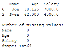
8.3 KNNImputer in Practice
Now we come to the last method described in this post for replacing missing values in practice.
8.3.1 Train-Test Split
df_practice_knn = df_practice.copy()
df_practice_knn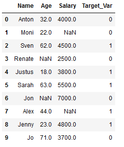
x = df_practice_knn.drop('Target_Var', axis=1)
y = df_practice_knn['Target_Var']

trainX, testX, trainY, testY = train_test_split(x, y, test_size = 0.2)
print()
print('trainX')
print()
print(trainX)
print('-------------------------')
print()
print('testX')
print()
print(testX)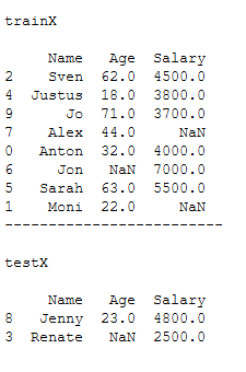
8.3.2 Fit&Transform (trainX)
# Fit and Transform trainX column 'Age' and 'Salary'
imp_age_salary_knn1 = KNNImputer(n_neighbors=2)
trainX[['Age', 'Salary']] = imp_age_salary_knn1.fit_transform(trainX[['Age', 'Salary']])

print(trainX)
print()
print('Number of missing values:')
print(trainX.isnull().sum())
pk.dump(imp_age_salary_knn1, open('imp_age_salary_knn1.pkl', 'wb'))8.3.3 Transform (testX)
I’ll leave out again the part about model training at this point, since it would only be fictitiously presented anyway.
testX.isnull().sum()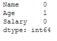
# Transform testX column 'Age' and 'Salary'
testX[['Age', 'Salary']] = imp_age_salary_knn1.transform(testX[['Age', 'Salary']])

print(testX)
print()
print('Number of missing values:')
print(testX.isnull().sum())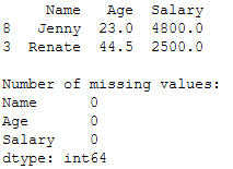
8.4 Recommendation
What works for me in practice is a method from statistics that can be used when the data of a variable is normally distributed.
We know from normal distributions (Bell Curve) that 68% of the data lie between Z-1 and Z1.
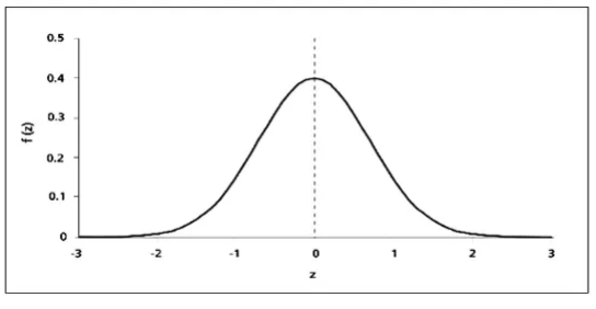
Source: SimplyPsychology
That is, they have a mean value of 0 +- 1sd with a standard normal distribution.

Source: SimplyPsychology
Therefore, for a variable with a normal distribution, we can replace the missing values with random values that have a range from mean - 1sd to mean + 1sd.
This method, is a little more cumbersome than the functions we used before, but it provides slightly more accurate values.
df_recom = df_knn.copy()
df_recom = df_recom[['Name', 'Age']]
df_recom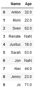
mean_age = df_recom['Age'].mean()
sd_age = df_recom['Age'].std()

print('Mean of columne "Age": ' + str(mean_age))
print('Standard deviation of columne "Age": ' + str(sd_age))
Fast saving of the values:
pk.dump(mean_age, open('mean_age.pkl', 'wb'))
pk.dump(sd_age, open('sd_age.pkl', 'wb'))
With the random.uniform function I can output floats for a certain range.
random.uniform(mean_age-sd_age,
               mean_age+sd_age)

print('Lower limit of the range: ' + str(mean_age-sd_age))
print('Upper limit of the range: ' + str(mean_age+sd_age))
def fill_missings_gaussian_func(col, mean, sd):
    if np.isnan(col) == True:
        col = random.uniform(mean-sd, mean+sd)
    else:
         col = col
    return col
df_recom['Age'] = df_recom['Age'].apply(fill_missings_gaussian_func, args=(mean_age, sd_age))
df_recom
Voilá, we have inserted different new values for the missing values of the column ‘Age’, which are between the defined upper and lower limit of the rage. Now, if you want to be very precise, you can round the ‘Age’ column to whole numbers to make it consistent.
9 Conclusion
In this post, I have shown different methods of replacing missing values in a dataset in a useful way. Furthermore, I have shown how these procedures should be applied in practice during a model training.