1 Introduction
Data manipulation is an elementary component in the data science field that requires the most time, among other things. It is therefore worthwhile to be fit in this discipline.
For this post the dataset flight from the statistic platform “Kaggle” was used. You can download it from my GitHub Repository.
import pandas as pd
import numpy as np
flight = pd.read_csv("path/to/file/flight.csv")2 Index
If you’ve worked with R before, you may not be used to working with an index. This is common in Python.
2.1 Resetting index
df = pd.DataFrame({'A': [1, 2, 3], 'B': [4, 5, 6]}, index=['a', 'b', 'c'])
df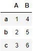
df = df.reset_index()
df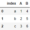
df.rename(columns ={df.columns[0]: 'ABC'}, inplace = True)
df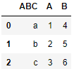
df.index.tolist()
df['A'].tolist()
2.2 Resetting multiindex
# Create a multiindex


index = pd.MultiIndex.from_product([[2013, 2014], [1, 2]],
                                   names=['year', 'visit'])
columns = pd.MultiIndex.from_product([['Bob', 'Guido', 'Sue'], ['HR', 'Temp']],
                                     names=['subject', 'type'])


data = np.round(np.random.randn(4, 6), 1)
data[:, ::2] *= 10
data += 37

# create the DataFrame
health_data = pd.DataFrame(data, index=index, columns=columns)
health_data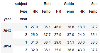
health_data.columns = health_data.columns.droplevel()
health_data = health_data.reset_index()
health_data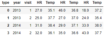
2.3 Setting index
Here we have the previously created data frame.
df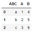
Now we would like to set an index again.
df.set_index([pd.Index([1, 2, 3])])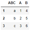
df.set_index('ABC')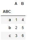
df.set_index(['A', 'B'])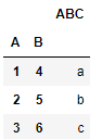
3 Modifying Columns
3.1 Rename Columns
show_rename = pd.DataFrame({'Name': ['1.Anton', '2.Susi', '3.Moni', '4.Renate'],
                   'Alter': [32,22,62,44],
                   'Gehalt': [4700, 2400,4500,2500]})
show_rename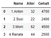
show_rename.rename(columns ={show_rename.columns[2]: 'Monatsgehalt'}, inplace = True)
show_rename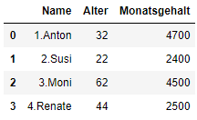
show_rename = show_rename.rename(columns={'Name':'Mitarbeiter', 'Alter':'Betriebszugehörigkeit'})
show_rename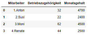
show_rename.columns = ['MA', 'Bzghk.', 'MGe.']
show_rename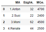
3.1.1 add_prefix
show_prefix = show_rename.copy()
show_prefix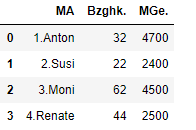
show_prefix.add_prefix('alte_MA_')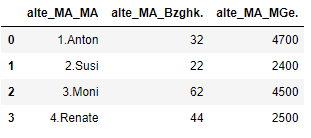
3.3 Add columns
data = {'country': ['Italy','Spain','Greece','France','Portugal'],
        'popu': [61, 46, 11, 65, 10],
        'percent': [0.83,0.63,0.15,0.88,0.14]}

df_MC = pd.DataFrame(data, index=['ITA', 'ESP', 'GRC', 'FRA', 'PRT'])
df_MC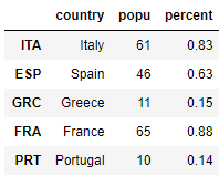
Add a list as a new column
df_MC['capital city'] = ['Rome','Madrid','Athens','Paris','Lisbon']
df_MC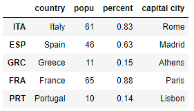
Add an array as a new column
ar = np.array([39,34,30,33,351])
ar
df_MC['Calling code'] = ar
df_MC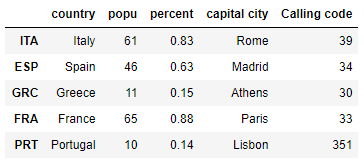
Add a Series array as a new column. When adding a Series data are automatically aligned based on index.
ser = pd.Series(['es','it','fr','pt','gr'], index = ['ESP','ITA','FRA','PRT','GRC'])
df_MC['Internet domain'] = ser
df_MC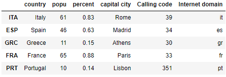
3.4 Drop and Delete Columns
The drop-function don’t delete columns.
df_MC.drop(columns=['country', 'popu', 'percent'])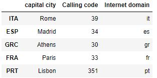
df_MC.head(2)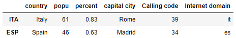
But del-function does this
del df_MC['Internet domain']
df_MC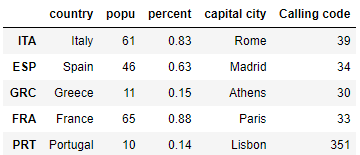
For multiple deletion use drop-function + inplace = True
df_MC.drop(["popu", "percent", "Calling code"], axis = 1, inplace = True)
df_MC.head(3)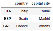
3.5 Insert Columns
Now I want to have my previously deleted column “Internet domain” back at a certain point.
ser = pd.Series(['es','it','fr','pt','gr'], index = ['ESP','ITA','FRA','PRT','GRC'])
#previously created syntax
df_MC.insert(1,'Internet domains',ser)
df_MC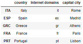
3.6 Rearrange Columns
clist = ['capital city','Internet domains','country']
df_MC = df_MC[clist]
df_MC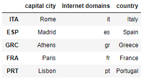
You can also simply move the last column to the front. This is often the case, for example, when you make predictions, which you would like to put in the original dataframe and usually in the first place.
cols = list(df_MC.columns)
cols = [cols[-1]] + cols[:-1]
df_MC = df_MC[cols]
df_MC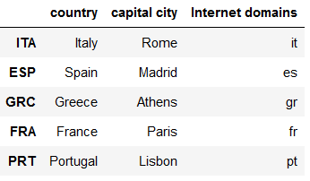
4 Modifying Rows
# Preparations

df =(
    flight
    .groupby(['Origin_Airport'])
    .agg({'Scheduled_Departure': 'mean',
          'Dep_Delay': 'mean',
          'Scheduled_Arrival': 'mean',
          'Arrival_Delay': 'mean'})
    .rename(columns={"Scheduled_Departure": "avg_Scheduled_Departure",
                    "Dep_Delay": "avg_Dep_Delay",
                    "Scheduled_Arrival": "avg_Scheduled_Arrival",
                    "Arrival_Delay": "avg_Arrival_Delay"})
    .reset_index()
)

df.head(5)
4.1 Round each column
df.round(2).head(2)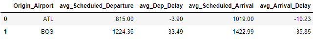
4.2 Round columns differently within a df
df.round({'avg_Scheduled_Departure': 1,
          'avg_Dep_Delay': 2,
         'avg_Scheduled_Arrival':3,
         'avg_Arrival_Delay':4}).head(2)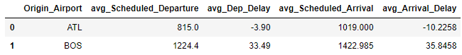
decimals = pd.Series([1, 2, 3, 4], index=['avg_Scheduled_Departure', 'avg_Dep_Delay', 'avg_Scheduled_Arrival', 'avg_Arrival_Delay'])
df.round(decimals).head(2)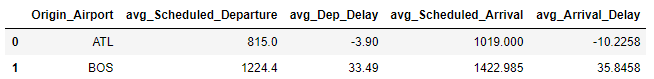
4.3 Drop Duplicates
To get clean data it is often necessary to remove duplicates. We can do so with the drop_duplicates function. Have a look at this dataframe:
df_duplicates = pd.DataFrame({'Case': [1,2,3,4,5],
                   'Value': [5,5,5,7,8]})
df_duplicates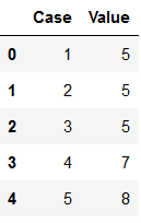
As we can see, there are several identical values in the ‘Value’ column. We do not want to have them like this. With keep=‘first’ we consider only the first value as unique and rest of the same values as duplicate.
df_subset_1 = df_duplicates.drop_duplicates(subset=['Value'], keep='first')
df_subset_1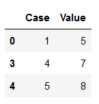
With keep=‘last’ we consider only the last value as unique and rest of the same values as duplicate.
df_subset_2 = df_duplicates.drop_duplicates(subset=['Value'], keep='last')
df_subset_2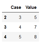
With keep=False we consider all of the same values as duplicates.
df_subset_3 = df_duplicates.drop_duplicates(subset=['Value'], keep=False)
df_subset_3
With the drop_duplicates function there is one more parameter that can be set: inplace. By default this is set to False. If we set this to True, the record does not have to be assigned to a separate object (as we have always done before).
df_duplicates.drop_duplicates(subset=['Value'], keep=False, inplace=True)

df_duplicates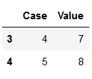
5 Replacing Values
5.1 One by One
df = flight[['DayOfWeek']]
df = df.replace(5, 'Friday')
df = df.replace(6, 'Saturday')
#and so on ...
df.head(5)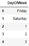
5.2 Collective replacement
df = flight[['DayOfWeek']]
vals_to_replace = {1:'Monday', 2:'Tuesday', 3:'Wednesday', 4:'Thursday', 5:'Friday', 6:'Saturday', 7:'Sunday'}

df['DayOfWeek'] = df['DayOfWeek'].map(vals_to_replace)
df.head()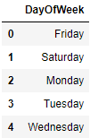
5.3 Conditional replacement
For an example of conditional replacement have a look at this dataframe:
df = pd.DataFrame({'Name': ['Anton', 'Anton', 'Moni', 'Moni', 'Justus'],
                   'Alter': [32,22,np.NaN,62,18],
                   'Gehalt': [np.NaN, np.NaN,np.NaN,np.NaN,500]})
df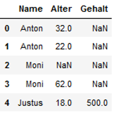
We want to check the names where the column ‘Gehalt’ is NaN.
df[df["Gehalt"].isnull() & (df["Name"] == 'Anton')]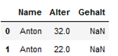
Here we go ! Now we want to replace exspecially these NaNs with a salary of 2.000 for Anton.
df['Gehalt'] = np.where((df.Name == 'Anton'), 2000, df.Gehalt)
df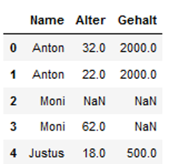
We can also use multiple conditions for filtering and replacement.
The code below shows a selection of the name (here Moni) for which no age is available. Now we want to replaces the NaNs for the salary.
df['Gehalt'] = np.where((df.Name == 'Moni') & (df.Alter.isna()), 3000, df.Gehalt)
df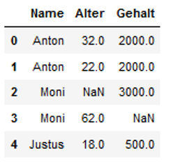
Finally we replace the hits that we find under Moni with an age greater than 50.
df['Gehalt'] = np.where((df.Name == 'Moni') & (df.Alter > 50), 4000, df.Gehalt)
df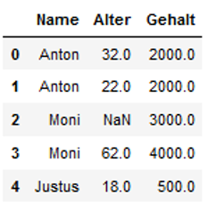
6 Function for colouring specific values
I always find it quite nice to be able to color-modify Python’s output so that you can immediately see important figures.
6.1 highest values
Sometimes it is useful, e.g. when you want to compare the performance values of algorithms during model training, the highest values are displayed in color.
colouring_df = pd.DataFrame({'Col1': [32,22,17,44],
                             'Col2': [32,22,62,28],
                             'Col3': [4700, 2400,4500,2500]})
colouring_df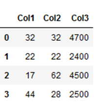
colouring_df.style.highlight_max(color = 'lightgreen', axis = 0)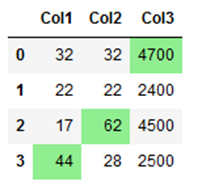
6.2 lowest values
Likewise, you can have even the lowest values displayed in color:
colouring_df.style.highlight_min(color = 'lightgreen', axis = 0)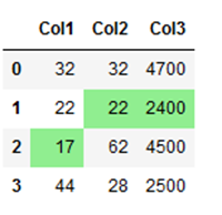
6.3 highest-lowest values
If you want to highlight values from different columns with different conditions, you can do this as follows:
colouring_df.style.highlight_max(axis=0,
                                color = 'lightgreen',
                                subset=['Col1',
                                        'Col2']).highlight_min(axis=0,
                                                               color = 'lightgreen',
                                                               subset=['Col3'])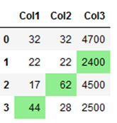
Here I have highlighted the highest values from columns ‘Col1’ and ‘Col2’ and the lowest value from column ‘Col3’.
6.4 negative values
Here is an example of how to highlight negative values in a data set:
negative_values_df = pd.DataFrame({'Col1': [-32,22,-62,44],
                                   'Col2': [32,-22,62,-44],
                                   'Col3': [-4700, 2400,-4500,2500]})
negative_values_df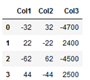
# Function for colouring(negative values red and positive values black)

def highlight_neg_values(s):
    if s.dtype == np.object:
        is_neg = [False for _ in range(s.shape[0])]
    else:
        is_neg = s < 0
    return ['color: red;' if cell else 'color:black'
            for cell in is_neg]

negative_values_df.style.apply(highlight_neg_values)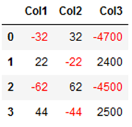
7 Conclusion
This was a small insight into the field of data manipulation. In subsequent posts, the topics of string manipulation and the handling of missing values will be shown.