1 Introduction
Never stop learning !
The entry into the field of data science with “R / R-Studio” was a smart matter. Now it’s time and for each Data Scientist advisable to learn another scripting language.
Let’s start with Python!
For this post the dataset flight from the statistic platform “Kaggle” was used. You can download it from my GitHub Repository.
2 Loading the libraries and the data
import pandas as pd
import numpy as np
flight = pd.read_csv("flight.csv")3 Overview of the data
With the following commands it is possible to get a quick overview of his available data.
flight.head()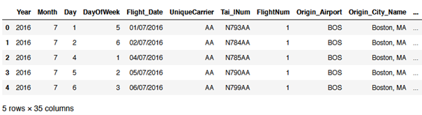
flight.tail()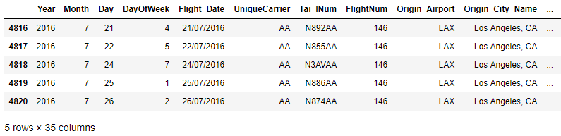
flight.shape
flight.columns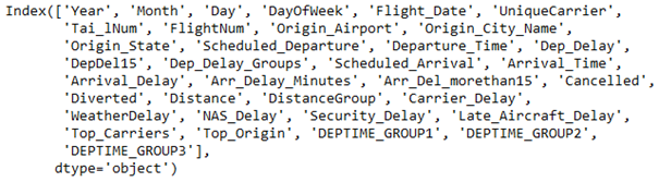
flight['Origin_Airport'].value_counts().head().T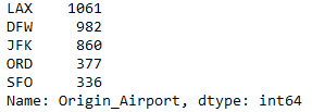
flight.dtypes.head()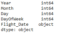
We can also output the unique values of a column.
#List unique values in the flight['Origin_Airport'] column
flight.Origin_Airport.unique()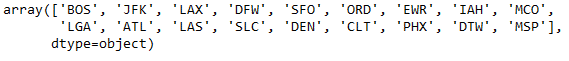
Now let’s take a look at the unique values of several columns. For this purpose, I will select 4 categorical columns from the data set as an example:
flight_subset = flight[['UniqueCarrier','Tai_lNum','Origin_Airport','Origin_City_Name']]
flight_subset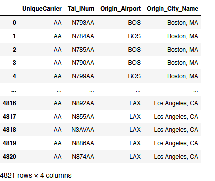
Now I can use a for loop to display the number of contained labels:
for feature in flight_subset.columns[:]:
    print(feature, ':', len(flight_subset[feature].unique()), 'labels')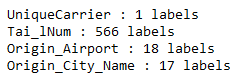
4 Get some statistics
flight.describe()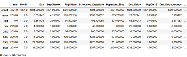
flight['Dep_Delay'].agg(['mean', 'median', 'std', 'min', 'max']).reset_index()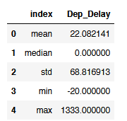
flight[['Origin_Airport', 'Departure_Time', 'Dep_Delay', 'Carrier_Delay']].groupby('Origin_Airport').mean().head()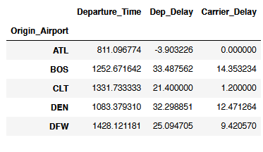
5 Select data
5.1 Easy Selection
flight[['Year']].head()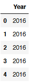
flight[['Year', 'WeatherDelay']].head()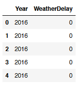
# Select specific rows
flight[1:4]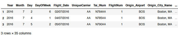
# Select specific rows & columns
flight.loc[1:4, ['Year', 'WeatherDelay', 'Flight_Date']]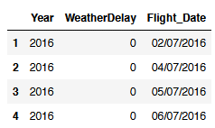
# Select all columns from Col_X to Col_Y
flight.loc[:,'Year':'DayOfWeek'].head()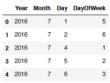
# Select all columns from Col_X to Col_Y and Col_Z
flight.loc[:,'Year':'DayOfWeek'].join(flight.loc[:,'Tai_lNum']).head()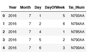
# Select all columns from Col_X to Col_Y and from Col_Z to Col_*
flight.loc[:,'Year':'DayOfWeek'].join(flight.loc[:,'Tai_lNum':'Origin_Airport']).head()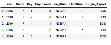
5.2 Conditional Selection
flight[(flight["Distance"] >= 3000) & (flight["DayOfWeek"] == 1) & (flight["Flight_Date"] == '11/07/2016')]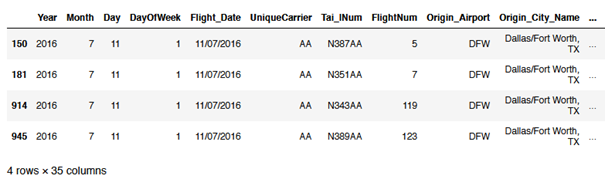
flight[(flight.Origin_Airport == 'ATL') | (flight.Origin_Airport == 'BOS')]['Origin_Airport']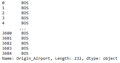
# If you want to see how many cases are affected use Shape[0]

flight[(flight["Distance"] >= 3000)].shape[0] 
5.3 Set option
With the set option function one can determine, how many lines and columns should be issued.
flight.head()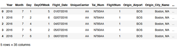
pd.set_option('display.max_rows', 2)
pd.set_option('display.max_columns', 2)
flight.head(200)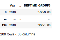
# Don't forget to reset the set options if they are no longer required.

pd.reset_option('all')
6 Dropping Values
6.1 Dropping Columns
df = pd.DataFrame({'Name': ['Anton', 'Moni', np.NaN, 'Renate', 'Justus'],
                   'Age': [32,22,62,np.NaN,18],
                   'Salary': [np.NaN, np.NaN,4500,2500,3800],
                   'Job': ['Student', np.NaN, 'Manager', 'Teacher', 'Student']})
df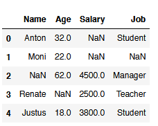
reduced_df = df.drop(['Job'], axis=1)
reduced_df.head()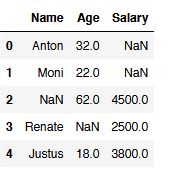
reduced_df2 = df.drop(['Salary', 'Job'], axis=1)
reduced_df2.head()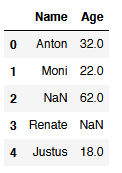
# You can also use a list to excluede columns
col_to_exclude = ['Salary', 'Job']

reduced_df_with_list = df.drop(col_to_exclude, axis=1)
reduced_df_with_list.head()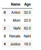
6.2 Dropping NaN Values
df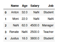
#Dropping all NaN values from column 'Name'
df.dropna(subset=['Name'])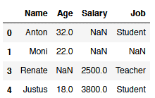
#Dropping all NaN values from the columns 'Salary' and 'Job' if there is min. 1
df.dropna(subset=['Salary', 'Job'])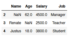
6.3 NaN Values vs. Null Values
NaN values and zero values are not the same thing. This becomes clear from the examples below, so that you do not mistakenly follow a false assumption.
df_NaN_vs_Null = pd.DataFrame({'AIRLINE': ['AS', 'LH', 'KE'],
                               'VALUE': [1, 0, np.NAN]})
df_NaN_vs_Null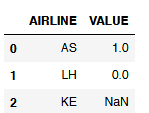
# The isna() function does its job well
df_NaN_vs_Null[df_NaN_vs_Null['VALUE'].isna()]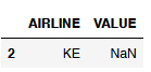
# The isnull() function also looks for NaN values not for NULL values!
df_NaN_vs_Null[df_NaN_vs_Null['VALUE'].isnull()]
# For Null values you have to select the respective column like this:
df_NaN_vs_Null[(df_NaN_vs_Null["VALUE"] == 0)]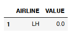
# If you are looking for both (NaN and Null Values) use this method:
df_NaN_vs_Null[(df_NaN_vs_Null["VALUE"] == 0) | (df_NaN_vs_Null["VALUE"].isnull())]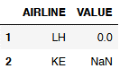
7 Filtering Values
Let’s use this dummy dataset:
df = pd.DataFrame({'Name': ['Maria', 'Marc', 'Julia', 'Mike', 'Sarah',
                            'Sven', 'Mel', 'Alex', 'John', 'Marlene'],
                   'Favorite_Fruit': ['Banana', 'Apple', 'Melon', 'Peach', 'Grape',
                                      'Melon', 'Orange', 'Banana', 'Melon', 'Apple']})
df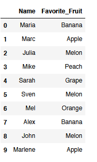
7.1 Filter with Lists
value_list = ["Apple", "Melon"]

boolean_value_list = df['Favorite_Fruit'].isin(value_list)
filtered_df = df[boolean_value_list]
filtered_df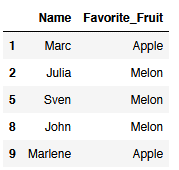
7.2 Exclude certain values
value_list = ["Apple", "Melon"]

inverse_boolean_value_list = ~df.Favorite_Fruit.isin(value_list)
inverse_filtered_df = df[inverse_boolean_value_list]
inverse_filtered_df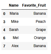
8 Working with Lists
8.1 Creation of Lists
df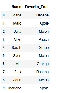
# Getting a list of unique values from a specific column

unique_list = df['Favorite_Fruit'].unique().tolist()
unique_list
# If you would like to get a list of the columns within a df use the to_list() function

column_list = df.columns.to_list()
column_list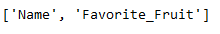
8.2 Comparing Lists
list_A = ['A',
          'B', 'C', 'D']

list_B = ['B', 'C', 'D',
          'E']
# Elements in A not in B
filtered_list = list(set(list_A) - set(list_B))
filtered_list
# Elements in B not in A
filtered_list = list(set(list_B) - set(list_A))
filtered_list
# Elements that occur in both lists (common elements)
filtered_list = list(set(list_A).intersection(list_B))
# Also works: filtered_list = list(set(list_B).intersection(list_A))

filtered_list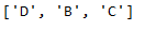
# Elements that just occur in one of both lists (not common elements)
filtered_list = list(set(list_A) ^ set(list_B))
filtered_list
9 Conclusion
Data wrangling is one of the most important disciplines in the field of data science. This was just a small sample of what is possible.